Timeline Options in Excel – Instructions

Timeline Options in Excel: Video Lesson

            This video lesson, titled “Excel for Microsoft 365 Tutorial: How to Modify Timelines in Excel,” shows how to apply timeline options in Excel. This video lesson is from our complete Excel tutorial, titled Mastering Excel Made Easy™.

Overview:

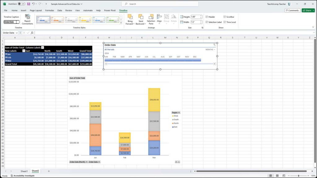
            This lesson shows you how to set timeline options in Excel. After inserting a timeline into a worksheet in Excel, a “Timeline” contextual tab then appears in the Ribbon. This tab appears in the Ribbon any time you select the timeline. You can use the buttons within this tab to modify the timeline settings and make other adjustments to it.

             In the “Timeline” button group at the left end of this tab, you can see and edit the name of the “Timeline Caption” within the text box. You can click the “Report Connections” button to open the “Report Connections” dialog box, where you can select the PivotTable and PivotChart reports to connect to the selected timeline by checking the checkboxes next to the names of the reports to filter with this timeline. Then click the “OK” button to apply your choices.

             In the “Timeline Styles” button group, you can click the style you wish to apply to your selected timeline to change its appearance. You can use the buttons within the “Arrange” button group to change the alignment and placement of the timeline pane in the worksheet.

            To set the size of the selected timeline pane, use the “Height” and “Width” fields within the “Size” button group. You can check or uncheck the checkboxes in the “Show” button group to show or hide the associated elements within the timeline.

Timeline Options in Excel: Instructions

1. To set timeline options in Excel, select the timeline to modify and click the “Timeline” contextual tab in the Ribbon.
2. To see and edit the name of the timeline, use the “Timeline Caption” text box in the “Timeline” button group at the left end of this tab.
3. If needed, to open the “Report Connections” dialog box to choose which reporting objects to associate with the timeline, click the “Report Connections” button in the “Timeline” button group.
4. Then select the PivotTable and PivotChart reports to connect to the selected timeline by checking the checkboxes next to their names and then clicking the “OK” button to apply your choices.
5. To change the appearance of the timeline, click the style to apply to the selected timeline in the “Timeline Styles” button group.
6. To change the alignment and placement of the timeline pane within the worksheet, use the buttons that appear within the “Arrange” button group.
7. If desired, to set the size of the selected timeline pane, use the “Height” and “Width” fields within the “Size” button group.
8. To show or hide elements within the timeline, check or uncheck the checkboxes for the associated elements in the “Show” button group.