Create a KPI in Power Pivot for Excel – Instructions

Create a KPI in Power Pivot for Excel: Video Lesson

            This video lesson, titled “Creating KPIs,” shows you how to create a KPI in Power Pivot for Excel. This video lesson is from our complete Excel tutorial, titled “Mastering Excel Made Easy v.2019 and 365.”

Create a KPI in Power Pivot for Excel: Overview

            Creating measures within the data model in Power Pivot then lets you create a KPI in Power Pivot for Excel. KPI stands for Key Performance Indicator. A KPI is a value, and often associated symbol, that gauges the performance of a base field in attaining a set value. Therefore, you must have three elements before you create a KPI in Power Pivot for Excel within a data model.

            First, you must have a base value. The base value is the measure to evaluate. Often, this is a simple aggregate function over a field. It is explicitly defined in the calculation area of the data model only to establish a base value within a KPI.

            Second, you must have a target value. This is often another measure within the calculation area. Alternatively, it can be an absolute value you enter when you create a KPI in Power Pivot for Excel.

            Third, you must define the status threshold within the KPI. This is the range between a low and high threshold that determines how well the base value met the target value. This often appears as a graphic in a PivotTable that shows the performance.

            For example, assume you have departmental budget information table with “Actual Expenses” and “Budgeted Expenses” fields. You could create a KPI in Power Pivot for Excel from the data in these fields. In this case, you define two measures in the calculation area of the table. Both measures are simple AutoSum values over the two columns. In this case, the =SUM([Actual Expenses]) measure is the base value. This value is then compared to the =SUM([Budgeted Expenses]) measure, the target value. You then set the status threshold of the KPI to 100%. This means the goal is to spend 100% of the budgeted amount.

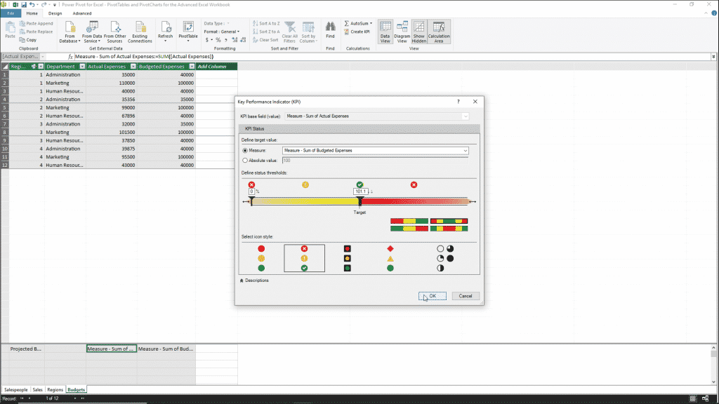
Create a KPI in Power Pivot for Excel – Instructions: A picture of the “Key Performance Indicator (KPI)” dialog box in Power Pivot for Excel.

            To create a KPI in Power Pivot for Excel after creating the necessary measure(s), select the measure that is the base value field for the KPI in the calculation area. Then click the “Home” tab within the Ribbon of the data model window. Then click the “Create KPI” button within the “Calculations” button group.

            In the “Key Performance Indicator (KPI)” dialog box that appears, the selected field appears at the top of the dialog box in the “KPI base field (value)” field. Next, in the “Define target value” section, select the desired option button for your KPI target value: “Measure” or “Absolute value.”

            If you select the “Measure” choice, select the name of the target value field you created from the adjacent drop-down menu. If you select “Absolute value,” enter the desired value into the adjacent field. Below that, in the “Define status thresholds” section, drag the percentage sliders into the desired locations. Then select a desired icon to represent these threshold values from the listing in the “Select icon style” section. When you are ready to create your KPI, click the “OK” button to finish.

            The KPI indicator appears as another type of field you can insert into the quadrants within the associated PivotTable. You can insert the “Value,” the “Goal,” or the “Status” of the KPI into the “Values” quadrant within the “PivotTable Fields” task pane.

Create a KPI in Power Pivot for Excel: Instructions

1. To create a KPI in Power Pivot for Excel, you need three things.
2. First, you must have a base value to evaluate. Often, this is a simple aggregate function over a field. It is explicitly defined in the calculation area of the data model only to establish a base value within a KPI.
3. Second, you must have a target value. This is often another measure within the calculation area. Alternatively, it can be an absolute value you enter when you create a KPI in Power Pivot for Excel.
4. Third, you must define the status threshold within the KPI. This is the range between a low and high threshold that determines how well the base value met the target value.
5. To create a KPI in Power Pivot for Excel after creating the necessary measure(s), select the measure that is the base value field for the KPI in the calculation area.
6. Then click the “Home” tab within the Ribbon of the data model window.
7. Then click the “Create KPI” button within the “Calculations” button group.
8. In the “Key Performance Indicator (KPI)” dialog box that appears, the selected field appears at the top of the dialog box within the “KPI base field (value)” field.
9. In the “Define target value” section, select the desired option button for your KPI target value: “Measure” or “Absolute value.”
10. If you select the “Measure” choice, select the name of the target value field you created from the adjacent drop-down menu.
11. If you select “Absolute value,” enter the desired value into the adjacent field.
12. Below that, in the “Define status thresholds” section, drag the percentage sliders into the desired locations.
13. Select a desired icon to represent these threshold values from the listing in the “Select icon style” section.
14. To create the KPI, click the “OK” button.
15. The KPI indicator appears as another type of field you can insert into the quadrants in the associated PivotTable. You can insert the “Value,” “Goal,” or “Status” of the KPI into the “Values” quadrant in the “PivotTable Fields” task pane.