Create Calculated Columns in Power Pivot in Excel – Instructions

Create Calculated Columns in Power Pivot in Excel: Video Lesson

            This video lesson, titled “Calculated Columns,” shows you how to create calculated columns in Power Pivot in Excel. This video lesson on how to create calculated columns in Power Pivot in Excel is from our complete Excel tutorial, titled “Mastering Excel Made Easy v.2019 and 365.”

Create Calculated Columns in Power Pivot in Excel: Overview

            This lesson shows you how to create calculated columns in Power Pivot in Excel. You can create calculated columns and measures from the tables in the Power Pivot data model. Doing this lets you create table values that you can then add to PivotTables and PivotCharts. This is one of the primary reasons to use the Power Pivot add-in, versus the standard PivotTables in Excel.

            There are many formulas in the Power Pivot data model that let you calculate values of the existing table columns. These formulas are not always exactly the same as the standard workbook formulas within Excel. These formulas are called DAX formulas. They sometimes use a slightly different function and syntax to calculate values than normal Excel functions. However, the syntaxes are very similar. Excel helps you create the DAX formulas for calculated columns and fields. That way, you won’t need to worry about the syntax of the formulas you create.

            You create calculated columns in Power Pivot in Excel within a table in the data model window to create a column value. You can then summarize that value within the PivotChart or PivotTable in the “Values” section. For example, if you had both a “Quantity” and “Unit Price” field in an “Order Details” table, you could create a new calculated column that displays the result of the product of these two columns as an “Order Total” calculated column. You could then add this column to the “Values” section of a PivotChart or PivotTable to find the sum of order totals for a given grouping.

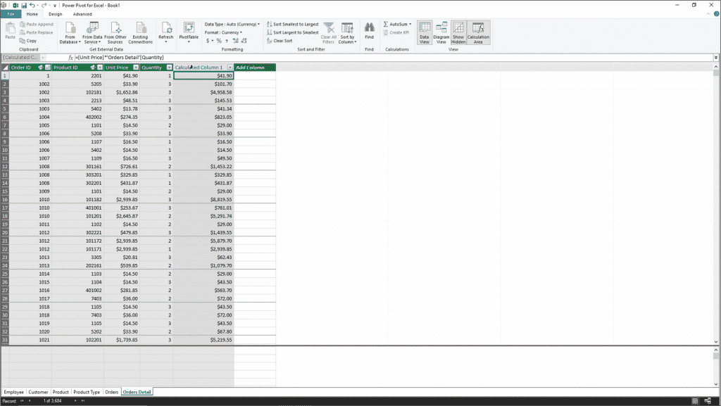
Create Calculated Columns in Power Pivot in Excel – Instructions: A picture of a user creating a calculated column in the data model window of Power Pivot in Excel by typing a simple formula.

            Alternatively, you could also create calculated columns in Power Pivot in Excel to derive a new column to use in the “Row” or “Columns” sections within a PivotTable or PivotChart. For example, if you had an “Order Date” field in an “Orders” table, but wanted to group results based on the quarter of the year in which the order was placed, you could create a calculated column in the table that displays the quarter of the year for each associated “Order Date” value. You could then add this new calculated column into the desired section within a PivotChart or PivotTable to group by its values.

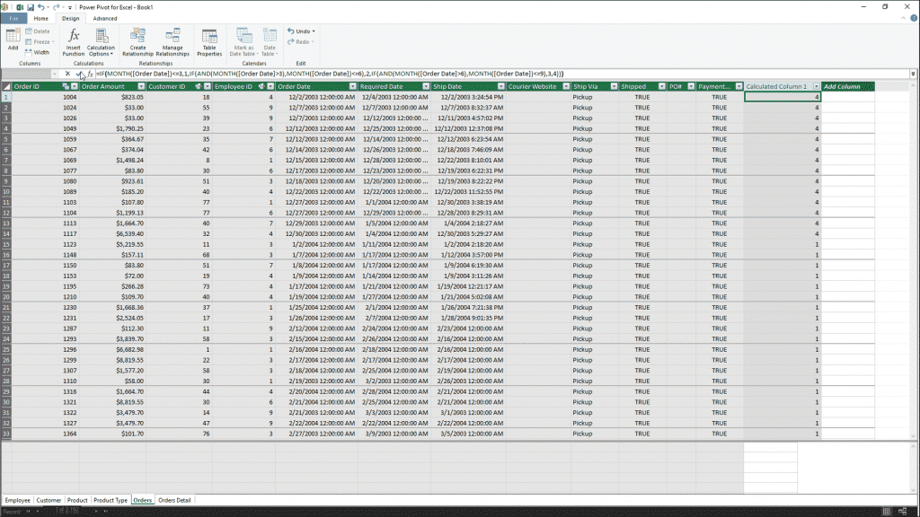
Create Calculated Columns in Power Pivot in Excel – Instructions: A picture of a user creating a calculated column in the data model window of Power Pivot in Excel which contains a formula that uses multiple functions.

            To create a calculated column in a table within the Power Pivot data model, first select the tab of the table in the data model window. Then click into the topmost cell within the “Add Column” column at the far right end of the table. Then enter the formula you want the column to calculate into the cell.

            For formulas you enter by hand, the formula appears within the Formula Bar. Start by typing the equal sign, followed by the field names, enclosed in brackets, and joined together by the standard mathematical operators. You can also simply click the field names of the fields in the table to add a field reference to the formula you enter. To accept the formula, click the checkmark button in the Formula Bar or press the “Enter” key on your keyboard.

            Alternatively, you can also create a formula that uses a function by clicking the “Design” tab in the Ribbon of the data model’s window. Then click the “Insert Function” button in the “Calculations” button group to open the “Insert Function” dialog box. This dialog box shows the functions you can insert. You can select a function in this listing. Doing that shows the function and its additional arguments at the bottom of the dialog box. Select a function to use and then click the “OK” button to insert it into the Formula Bar. Then finish entering the function’s additional arguments into the Formula Bar. To accept the formula, click the checkmark button in the Formula Bar or press the “Enter” key on your keyboard.

Create Calculated Columns in Power Pivot in Excel: Instructions

1. To create calculated columns in Power Pivot in Excel, select the tab of the table in the Power Pivot data model window within which to create the calculated column.
2. Click into the topmost cell within the “Add Column” column at the far right end of the table.
3. Enter the formula you want the column to calculate into the selected field.
4. For formulas you enter by hand, the formula appears within the Formula Bar. Start by entering the equal sign, followed by the field names, enclosed in brackets, and joined together by the standard mathematical operators. You can also simply click the field names of the fields in the table to add a field reference to the formula you enter.
5. To accept the formula, click the checkmark button in the Formula Bar or press the “Enter” key on your keyboard.
6. Alternatively, to create a formula that uses a function, click the “Design” tab in the data model window’s Ribbon.
7. Then click the “Insert Function” button in the “Calculations” button group to open the “Insert Function” dialog box.
8. Then select a function in the listing in this dialog box.
9. Doing that shows the function and its additional arguments at the bottom of the dialog box.
10. After selecting the desired function, then click the “OK” button to insert it into the Formula Bar.
11. Then finish entering the function’s additional arguments into the Formula Bar.
12. To accept the formula, click the checkmark button in the Formula Bar or press the “Enter” key on your keyboard.