Excel 2013 allows you to create charts from the data stored in a worksheet more easily than in previous versions. Charts are useful for times when you wish to create visual representations of the worksheet data for meetings, presentations, or reports.
To insert a chart, first select the cell range that contains the data that will be used in the chart- including the row and column labels. This allows the selected data to automatically be used in the chart, saving you the step of having to select it later. You can also adjust your data selection later on, if needed, but selecting the data first allows you to see the previews of how the chart will appear once inserted much more clearly.
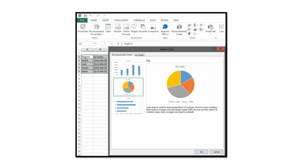
Next click the “Insert” tab in the Ribbon. In the “Charts” button group, you can see various types of charts that you can insert. Starting in Excel 2013, you can insert a chart by clicking the “Recommended Charts” button to open the “Insert Chart” dialog box and display the “Recommended Charts” tab. On this tab you will see the types of charts that Excel thinks would best illustrate your selected data. You can click on the choices shown at the left side of the tab to see a preview of the chart appear to the right. If you wish to insert one of the choices shown, click on it to select it from the listing at the left side of the tab and then click the “OK” button at the bottom of the “Insert Chart” dialog box.
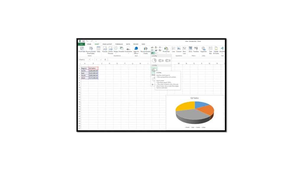
Another way to insert a chart based on selected data is to click on the button that represents the general chart type that you want to use within the “Charts” button group, and then click on the specific subtype to insert within the button’s drop-down menu.
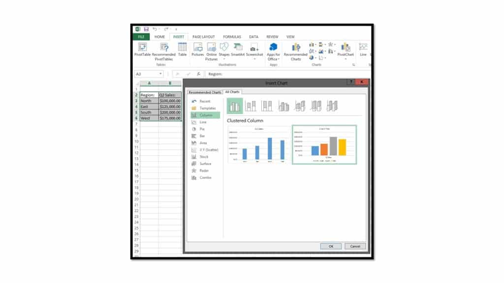
To view all of your charting choices and then insert a selected chart type, you can click the “See All Charts” button in the lower right corner of the “Charts” group to open the “Insert Chart” dialog box. To display all available chart choices, click the “All Charts” tab. On this tab you can select a major chart type from the listing shown at the left side of the dialog box. You can then select the specific subtype to insert by clicking on the desired subtype in the list at the right side of the dialog box. To then insert a chart of the selected subtype, you can click the “OK” button at the bottom of the dialog box.
Using any of these chart insertion methods will insert a chart of the selected subtype as an embedded chart object within the current worksheet. The next thing that you should immediately notice is that when you have a chart object selected, you will see a new contextual tab appear in the Ribbon. This is the “Chart Tools” tab, and it consists of two tabs: “Design” and “Format.” You will use the buttons within the various button groups on these two tabs that appear in the “Chart Tools” contextual tab to make changes to the selected chart objects.
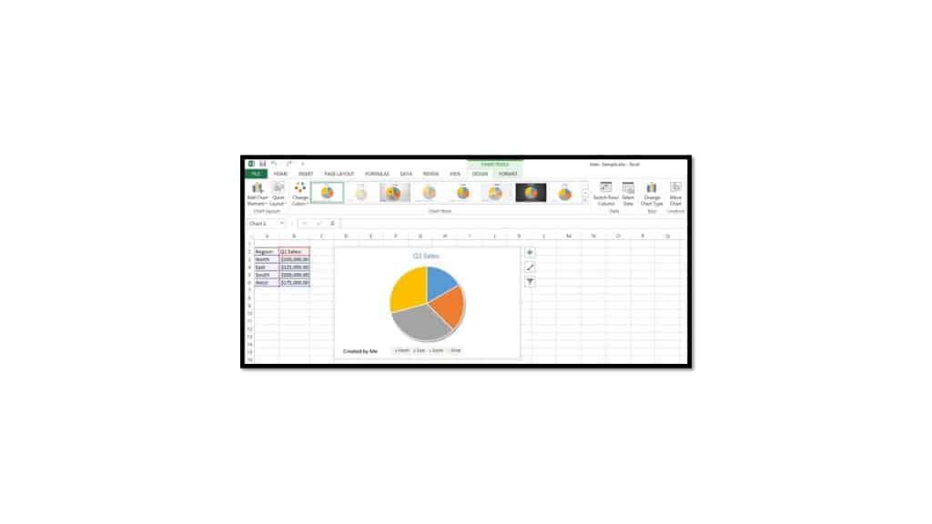 When a chart object is selected in Excel 2013, you will also now see a three-button grouping of chart options appear at the right side of the selected chart object. The buttons are, from top to bottom, “Chart Elements,” “Chart Styles,” and “Chart Filters.” You can also use these buttons to make changes to your selected chart object.