Format a PivotTable in Excel – Instructions and Video

Format a PivotTable in Excel: Video Lesson

            This video lesson, titled “Excel for Microsoft 365 Tutorial: How to Format PivotTables in Excel,” shows you how to format a PivotTable in Excel. This video lesson is from our complete Excel tutorial, titled Mastering Excel Made Easy™.

Overview

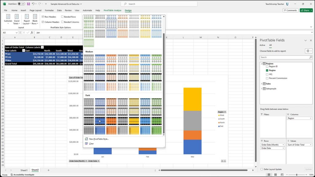
            To format a PivotTable in Excel, click into any cell in the PivotTable. To apply a PivotTable style, which applies preset formatting to PivotTables in Excel, then click the desired style to apply from the listing of PivotTable styles in the “PivotTable Styles” button group on the “Design” contextual tab in the Ribbon.

            If you want to modify the settings of the preset PivotTable styles, check the desired checkboxes in the “PivotTable Style Options” button group on the “Design” contextual tab in the Ribbon. Doing this lets you select the areas within the PivotTable to which to apply special formatting. To apply special formatting to the “Row Headers” and “Column Headers,” check those checkboxes. To apply banding to the rows or columns in the PivotTable, check the “Banded Rows” or “Banded Columns” checkboxes.

            If you want to change the summarization and layout of a PivotTable, use the buttons in the “Layout” button group on the “Design” contextual tab in the Ribbon. To choose a layout for subtotals in a selected PivotTable, click the “Subtotals” button and select a choice from its drop-down menu. To choose the display of grand totals in a selected PivotTable, click the “Grand Totals” button and select a choice from its drop-down menu.

            If you want to change the layout of a selected PivotTable, click the “Report Layout” button, and then select a choice from its drop-down menu. Finally, to choose how to show blank rows in a selected PivotTable, click the “Blank Rows” button and then select a choice from its drop-down menu.

Format a PivotTable in Excel: Instructions

1. To format a PivotTable in Excel, click into any cell within a PivotTable.
2. To use PivotTable styles to apply preset formatting to PivotTables in Excel, then click the desired style to apply from the listing of PivotTable styles in the “PivotTable Styles” button group on the “Design” contextual tab in the Ribbon.
3. If you want to modify the settings of the preset PivotTable styles, check the desired checkboxes in the “PivotTable Style Options” button group on the “Design” contextual tab in the Ribbon.
4. To apply special formatting to the “Row Headers” and “Column Headers,” check those checkboxes.
5. To apply banding to the rows or columns in the PivotTable, check the “Banded Rows” or “Banded Columns” checkboxes.
6. If you want to change the summarization and layout of a PivotTable, use the buttons in the “Layout” button group on the “Design” contextual tab in the Ribbon.
7. To choose a layout for subtotals in a selected PivotTable, click the “Subtotals” button and select a choice from its drop-down menu.
8. To choose the display of grand totals in a selected PivotTable, click the “Grand Totals” button and select a choice from its drop-down menu.
9. If you want to change the layout of a selected PivotTable, click the “Report Layout” button, and then select a choice from its drop-down menu.
10. Finally, to choose how to show blank rows in a selected PivotTable, click the “Blank Rows” button and then select a choice from its drop-down menu.