Format Trendlines in Excel Charts – Instructions

Format Trendlines in Excel Charts: Video Lesson

            This video lesson, titled “Excel for Microsoft 365 Tutorial: How to Format Chart Trendlines in Excel,” shows you how to format trendlines in Excel charts. This video lesson is from our complete Excel tutorial, titled “Mastering Excel Made Easy.”

Format Trendlines in Excel Charts: Overview

            You can easily format trendlines in Excel charts if you applied them to one or more chart series. To format trendlines in Excel if you applied trendlines to one or more series in a selected Excel chart, choose the desired trendline to format from the “Chart Elements” drop-down in the “Current Selection” button group on the “Format” contextual tab in the Ribbon. Then click the “Format Selection” button below the drop-down menu in the same button group.

            Alternatively, to format trendlines in Excel charts, right-click the trendline to format in the chart. Then select the “Format Trendline…” command from the pop-up menu that appears.

            Using either method then displays the “Format Trendline” task pane at the right side of the screen. In the “Trendline Options” category, which appears at the top of the pane and is selected by default, click the “Fill & Line,” “Effects,” or “Trendline Options” subcategory settings icon below the category to set its related options for the trendline.

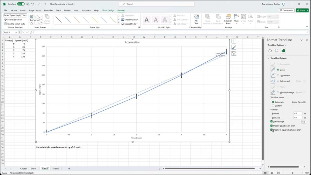
            The formatting options for the selected subcategory appear in collapsible and expandable lists at the bottom of the task pane. To expand and collapse the individual subcategory options, click the option titles. Then set any individual options, as desired, in the task pane to immediately apply those changes. When finished, click the “X” button in the upper-right corner of the task pane to close it.

Format Trendlines in Excel Charts: Instructions

1. To format a trendline in Excel if you applied trendlines to one or more series in an Excel chart, choose the desired trendline to format from the “Chart Elements” drop-down in the “Current Selection” button group on the “Format” contextual tab in the Ribbon.
2. Then click the “Format Selection” button below the drop-down menu in the same button group.
3. Alternatively, to format trendlines in Excel charts, right-click the trendline to format in the chart.
4. Then select the “Format Trendline…” command from the pop-up menu that appears.
5. Using either method then shows the “Format Trendline” task pane at the right side of the screen.
6. In the “Trendline Options” category, which appears at the top of the pane and is selected by default, click the “Fill & Line,” “Effects,” or “Trendline Options” subcategory settings icon below the category to set its related options for the trendline.
7. The formatting options for the selected subcategory appear in collapsible and expandable lists at the bottom of the task pane.
8. To expand and collapse the individual subcategory options, click the option titles.
9. Then set any individual options, as desired, in the task pane to immediately apply those changes.
10. When finished, click the “X” button in the upper-right corner of the task pane to close it.