Freeze Panes in Excel – Instructions and Video Lesson

Freeze Panes in Excel: Video Lesson

            This video lesson, titled “Freeze Panes,” shows how to freeze panes in Excel. This video lesson is from our complete Excel tutorial, titled “Mastering Excel Made Easy v.2019 and 365.”

Freeze Panes in Excel: Overview

            You can freeze panes in Excel to view data in two separate sections of a long worksheet simultaneously. You can freeze panes in Excel to freeze one or two sections of a worksheet to prevent scrolling. Then you can then scroll the unfrozen section of the worksheet to view two different worksheet sections at the same time.

            There are different ways to freeze panes in Excel. One way is to select the cell below the row and to the right of the column to freeze. Then click the “View” tab in the Ribbon. You then click the “Freeze Panes” button in the “Window” button group. Finally, choose the “Freeze Panes” command from the drop-down menu. After that, when you scroll through the worksheet, the information in the frozen panes will not scroll.

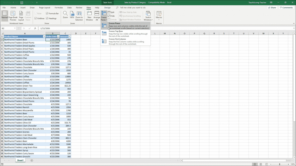
Freeze Panes in Excel – Instructions: A picture of a user selecting the Freeze Panes button in Excel.

            Notice the other choices shown in the drop-down menu after you click the “Freeze Panes” button. You can instead select the “Freeze Top Row” command to only freeze the top row in your worksheet. Alternatively, you can select the “Freeze First Column” command to freeze the first column in the worksheet. These command are useful for keeping column and row titles in view while looking at data in long workbooks.

            Note that the “Freeze Panes” command is a toggle command. This means you perform the same action to turn the “Freeze Panes” feature on or off. So, you can click the “Freeze Panes” button again and then choose “Unfreeze Panes” to turn it off.

Freeze Panes in Excel: Instructions

1. To freeze panes in both columns and rows in a worksheet, select the cell below the row and to the right of the column to freeze.
2. Click the “View” tab in the Ribbon.
3. Then click the “Freeze Panes” button in the “Window” button group.
4. Then choose the “Freeze Panes” command from the drop-down menu.
5. To freeze the top row of a worksheet, click the “View” tab in the Ribbon.
6. Then click the “Freeze Panes” button in the “Window” button group.
7. Then choose the “Freeze Top Row” command from the drop-down menu.
8. To freeze the first column of a worksheet, click the “View” tab in the Ribbon.
9. Then click the “Freeze Panes” button in the “Window” button group.
10. Then choose the “Freeze First Column” command from the drop-down menu.
11. To turn off the “Freeze Panes” feature, click the “View” tab in the Ribbon.
12. Then click the “Freeze Panes” button in the “Window” button group.
13. Then choose the “Unfreeze Panes” command from the drop-down menu.