Formatting cells in Excel can be a great way to add professionalism to an Excel spreadsheet. In can also be a great way to have numbers and figures in your charts stand out. In this post, we will discuss how to format cells in Microsoft Excel 2013.
1.Select the cells that you want to format.
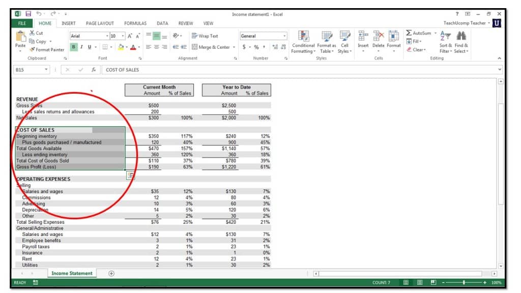
2.Click the desired buttons in the “Font,” “Alignment” or “Number” button groups on the “Home” tab in the Ribbon.
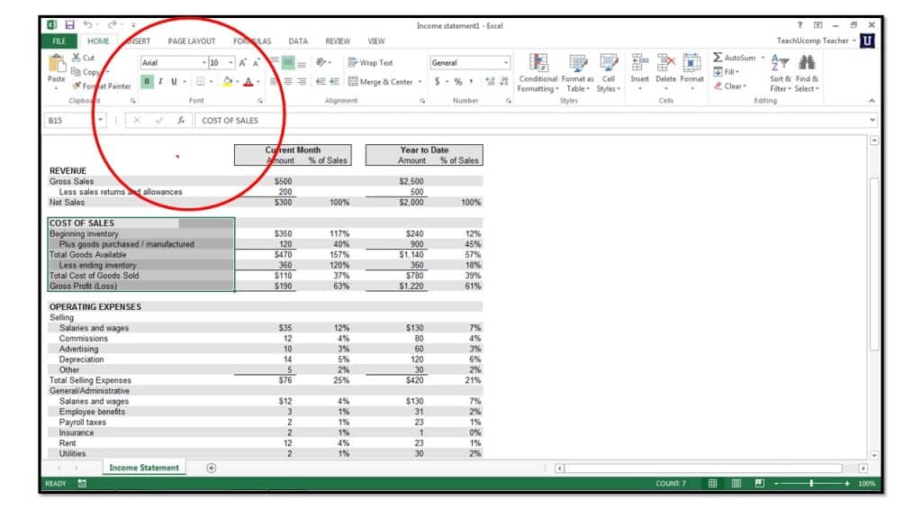
3. You can also use the tools and buttons available in the “Conditional Formatting” section to add formatting to cells.
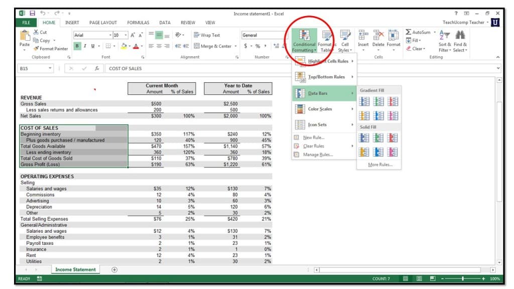
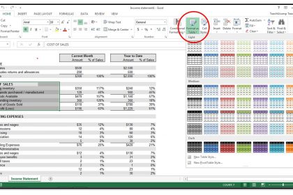
4. If you would like to format the cells as a table, select a choice from the “Format as Table” drop down.
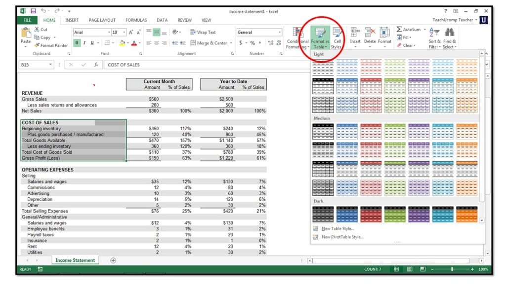
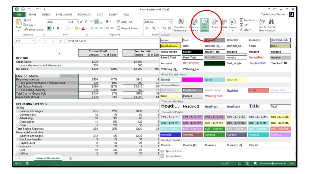
5. Finally, you can use the options available in the “Cell Styles” drop down to select specific cell styles.
