Name an Embedded Chart in Excel – Instructions

Name an Embedded Chart in Excel: Video Lesson

          This video lesson, titled “Excel for Microsoft 365 Tutorial: How to Name a Chart in Excel,” shows you how to name an embedded chart in Excel for Microsoft 365. This video lesson is from our complete Excel tutorial, titled Mastering Excel Made Easy™.

Overview:

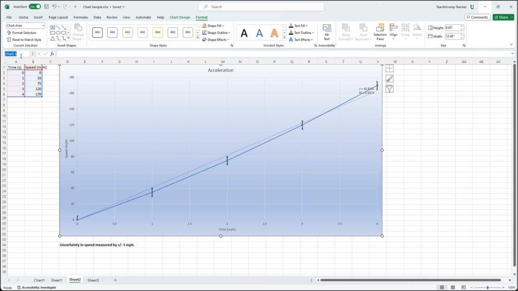
            You can easily name an embedded chart in Excel. To name a chart that is embedded within an Excel worksheet, first select the chart to name within a worksheet. You can then click into the “Name Box” at the left end of the Formula Bar. Then simply type a new name for your selected chart. After entering a chart name, then press the “Enter” key on your keyboard to apply it.

            By default, newly created charts in Excel get default names with numbers in the order in which they were created. This default chart name is not very descriptive or helpful if you want to refer to the chart later. Naming a chart in Excel allows you to more easily refer to the chart. This is especially true if you have multiple charts within your workbook. This also assists in giving the chart a name for use in VBA (Visual Basic for Applications) coding, if needed.

Name an Embedded Chart in Excel: Instructions

1. To name an embedded chart in Excel, select the chart to name within the worksheet.
2. Then click into the “Name Box” at the left end of the Formula Bar.
3. Then enter a new name for the selected chart.
4. After entering a chart name, then press the “Enter” key on your keyboard to apply it.