Outline Excel Data in Microsoft Excel – Instructions
Outline Excel Data in Microsoft Excel: Video Lesson
The video lesson above, titled “Applying and Removing Outlines,” shows how to outline Excel data. The following video, titled “Using Outlines,” shows you how to use outlines in Excel. These video lessons are from our complete Excel tutorial, titled “Mastering Excel Made Easy v.2019 and 365.”
Outline Excel Data in Microsoft Excel: Overview
You can outline Excel data to add an organizational quality to a long or wide worksheet. When you outline Excel data, you group worksheet data into different levels based on column and row headings. Lower level data is associated with the headings in the rows or columns. To outline Excel data, though, you must have a structured worksheet that would benefit from outlining. Usually, large worksheets that have column and row headings, detail data, and totals or subtotals can benefit from outlining.
Once applied, you can expand the outline to view any pertinent detail data. You can also collapse it to hide the detail data, but still show totals. This makes outlining larger, organized worksheets an excellent idea because it minimizes the scrolling needed to show the data you want to see. You can also see labels and totals that may normally be difficult to see simultaneously because of their separation within the worksheet’s columns and rows.
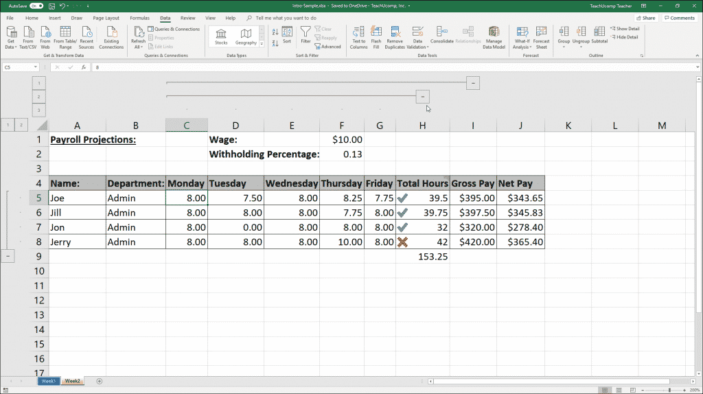
When an outlined section is expanded, you can see all of the data in that section. Also, a minus (-) sign appears above the section. If you click the minus sign, the section collapses, hiding the detail data. The minus sign also turns into a plus sign (+), indicating that there is hidden detail data. Clicking the plus sign expands the section again.
You may also click the small “1” and “2” numbers at the left end or top of the outline section to view the first level or second level of detail data. It is also possible to have multiple levels of outlining in the same section.
Outline Excel Data in Microsoft Excel – Instructions: A picture of an Excel worksheet with an outline applied.
To outline Excel data by applying an outline to a selected cell range, first select the cell range to outline. Then click the “Group” button in the “Outline” group on the “Data” tab in the Ribbon to launch the “Group” dialog box. In the “Group” dialog box, select whether to group the rows or columns of your cell selection. Then click the “OK” button to apply outline Excel data in the columns or rows.
To remove an outline, select the cell range to which you applied the outline. Then click the “Ungroup” button in the “Outline” group on the “Data” tab in the Ribbon. Doing this then opens the “Ungroup” dialog box, where you choose whether to ungroup the selection’s rows or columns. Then click the “OK” button to remove the outlining from the selection’s columns or rows.
You can also apply an auto outline to an entire worksheet. Just select any cell in the worksheet area. Then click the drop-down “Group” button in the “Outline” group on the “Data” tab in the Ribbon. Select the “Auto Outline” command from the drop-down menu of choices. The worksheet is automatically outlined, depending on the logical structure applied to the worksheet. This is a quick and easy way to outline an entire worksheet.
To remove an applied auto outline, click the “Data” tab in the Ribbon. Then click the drop-down “Ungroup” button in the “Outline” button group. Then select the “Clear Outline” command from the button’s drop-down menu. This will remove any outlining from your worksheet.
Outline Excel Data in Microsoft Excel: Instructions
- To collapse an outline, click the minus sign (-) in the gray outline border over the columns or next to the rows to collapse.
- To expand an outline, click the plus sign (+) in the gray outline border over the columns or next to the rows to expand.
- You may also click the small “1” and “2” numbers at the left end or top of the outlined section to view the first level or second level of detail data.
- To outline Excel data by applying an outline to a selected range of cells, select the cell range to outline.
- Then click the “Data” tab in the Ribbon.
- Then click the “Group” button in the “Outline” button group to launch the “Group” dialog box.
- In the “Group” dialog box, select whether to group the cell selection’s rows or columns.
- Then click the “OK” button to group the selected columns or rows.
- To remove an outline, select the outlined cell range and then click the “Data” tab in the Ribbon.
- Then click the “Ungroup” button in the “Outline” button group on to launch the “Ungroup” dialog box.
- In the “Ungroup” dialog box, select whether to ungroup the selection’s rows or columns.
- Then click the “OK” button to remove the outlining from the selection’s columns or rows.
- To apply an auto outline to an entire worksheet, select any cell in the worksheet area and then click the “Data” tab in the Ribbon.
- Then click the drop-down “Group” button in the “Outline” button group.
- Select the “Auto Outline” command from the drop-down menu of choices.
- To remove an auto outline you have applied, click the “Data” tab in the Ribbon.
- Then click the drop-down “Ungroup” button in the “Outline” button group.
- Then select the “Clear Outline” command from the button’s drop-down menu to remove any outlining from your worksheet.


