Split Panes in Excel – Instructions and Video Lesson

Split Panes in Excel: Video Lesson

            This video lesson, titled “Split Panes,” shows how to split panes in Excel. This video lesson is from our complete Excel tutorial, titled “Mastering Excel Made Easy v.2019 and 365.”

Split Panes in Excel: Overview

            To split panes in Excel when viewing a large worksheet, use the “Split” command in Excel. This command lets you split the Excel worksheet into different panes. Each pane contains its own horizontal and vertical scroll bars. Therefore, you can scroll each pane separately to view information from different sections of the worksheet. For example, you could split a large worksheet to see column headings in the top row and totals in the bottom row at the same time.

            To split a worksheet into four separately scrollable quadrants, first click to select the cell below and to the right of where you want the split to appear. Then click the “View” tab in the Ribbon. Then click the “Split” button in the “Window” button group to split the current worksheet into four separate panes. This lets you scroll each pane to independent sections of the same worksheet. You can click the “Split” button again to remove the split panes, when finished.

            To horizontally split a worksheet into two panes, click the gray row header (where the actual row number appears) of the row below where you want the split to appear. Alternatively, to vertically split a worksheet into two panes, click the gray column heading (where the actual column letters appear) of the column to the right of where you want the split to appear. After making either selection, then click the “View” tab in the Ribbon. Then click the “Split” button in the “Window” button group to split the worksheet. To turn it off, click into the worksheet and then click the same “Split” button again.

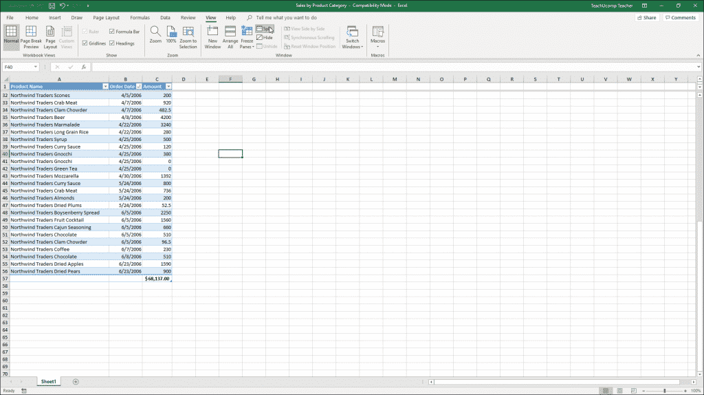
Split Panes in Excel – Instructions and Video Lesson: A picture of a large Excel workbook that is horizontally split into two separate panes.

            When a worksheet contains split panes in Excel, you can also move the splits. To do this, hover your mouse pointer over one of the light gray split lines until the mouse pointer turns into a double line intersected by a double-pointed arrow. Then click and drag in either direction shown by the arrows to move the split line to the desired location. Then release your mouse button when it is in the desired position.

Split Panes in Excel: Instructions

1. To split a worksheet into four separately scrollable quadrants, click to select the cell below and to the right of where you want the split to appear.
2. Then click the “Split” button in the “Window” button group on the “View” tab in the Ribbon.
3. To remove the split panes when finished, click the “Split” button again.
4. To horizontally split a worksheet into two panes, click the gray row header (where the actual row number appears) of the row below where you want the split to appear.
5. Alternatively, to vertically split a worksheet into two panes, click the gray column heading (where the actual column letters appear) of the column to the right of where you want the split to appear.
6. After making either selection, then click the “View” tab in the Ribbon.
7. Then click the “Split” button in the “Window” button group to split the worksheet.
8. To turn it off, click into the worksheet and then click the same “Split” button again.
9. To move the split lines within a worksheet that contains split panes, hover your mouse pointer over one of the light gray split lines until the mouse pointer turns into a double line intersected by a double-pointed arrow.
10. Then click and drag in either direction shown by the arrows to move the split line to the desired location.
11. Then release your mouse button when it is in the desired position.