Use a Top 10 AutoFilter in Excel – Instructions
Use a Top 10 AutoFilter in Excel: Video Lesson
This video lesson, titled “Using the Top 10 AutoFilter,” shows you how to use a Top 10 AutoFilter in Excel. This video lesson is from our complete Excel tutorial, titled “Mastering Excel Made Easy v.2019 and 365.”
Use a Top 10 AutoFilter in Excel: Overview
You can use a Top 10 AutoFilter in Excel to show a specified number of the top or bottom percent or items in a field within the table. When you use a Top 10 AutoFilter in Excel, it defaults to showing the top 10 percent of a column. However, you could also change it to show you the bottom 5 items by value within a column, too. Note that you cannot use a Top 10 AutoFilter in Excel on text fields. This is because text fields have no numeric ranking by which to base a value.
To use a Top 10 AutoFilter in Excel, click the AutoFilter drop-down arrow button next to the column heading for the field by which to filter the table. Next, roll down to the “Number Filters” choice. Then select the “Top 10…” option from the side menu that appears to open the “Top 10 AutoFilter” dialog box.
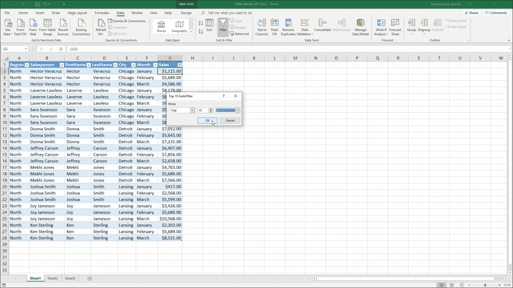
Use a Top 10 AutoFilter in Excel – Instructions: A picture of the “Top 10 AutoFilter” dialog box in Excel.
In this dialog box, select the first drop-down and pick either the “Top” or “Bottom” choice. Next, enter a number into the spinner box in the center of the dialog box. Finally, use the drop-down to the right to pick either the “Items” or “Percent” choice.
The criteria that then appears across the dialog box is the filter setting you will apply to the selected column. So, you could view only the “Top 10 Items” or “Bottom 40 Percent” or any other variation using this dialog box. When you have created the desired filter, just click “OK” to apply it.
Use a Top 10 AutoFilter in Excel: Instructions
- To use a Top 10 AutoFilter in Excel, click the AutoFilter drop-down arrow button next to the column heading for the field by which to filter the table.
- Roll your mouse down to the “Number Filters” choice.
- Select the “Top 10…” option from the side menu that appears.
- In the “Top 10 AutoFilter” dialog box, select the first drop-down and pick either the “Top” or “Bottom” choice.
- Enter a number into the spinner box in the center of the dialog box.
- Use the drop-down to the right to pick either the “Items” or “Percent” choice.
- The criteria that then appears across the dialog box is the filter setting you will apply to the selected column.
- When you have created the desired filter, click “OK” to apply it.