Conditional Formatting in Excel – Instructions

by Joseph Brownell / Wednesday, October 09 2019 / Published in Excel 2013, Excel 2016, Excel 2019, Excel for Office 365, Latest, Microsoft, Office 2013, Office 2016, Office 2019, Office 365

Conditional Formatting in Excel: Video Lesson

This video lesson, titled “Conditional Formatting,” shows you how to apply conditional formatting in Excel. This video lesson is from our complete Excel tutorial, titled “Mastering Excel Made Easy v.2019 and 365.”

Conditional Formatting in Excel: Overview

Conditional formatting in Excel lets you define criteria for cells which change the way the cells look in the worksheet, but only if the cells’ values match the criteria. For example, you could create a conditional formatting criterion that makes a worksheet cell appear with a red fill color only if it contains a negative number. You can apply conditional formatting in Excel to all types of cells. However, it is very helpful for visually changing the display of formula cells based on their values, which may change due to data entry.

You can apply several preset conditional formatting rules in Excel. Alternatively, you can create your own rules and formatting to apply. To apply conditional formatting in Excel, first select the worksheet cells to which to apply conditional formatting. Then click the “Conditional Formatting” button in the “Styles” button group on the “Home” tab of the Ribbon.

To apply a preset conditional format using the selected cells’ values as the conditional formatting criterion’s upper and lower bounds, then simply roll down to the conditional formatting style to use in the second section of the drop-down menu that appears. From the side menu that appears, then click to choose the specific style variation to apply to the selected cells.

Alternatively, to create custom conditional formatting rules that let you define the cell criteria and associated formatting to apply, select one of the rule choices in the first section of the drop-down menu. You can select either the “Highlight Cell Rules” or “Top/Bottom Rules” choice. From the side menu that then appears, select the type of values to highlight. Doing this opens a dialog box where you enter the criteria, which when met, applies the formatting you then choose. Then click the “OK” button to create the rule.

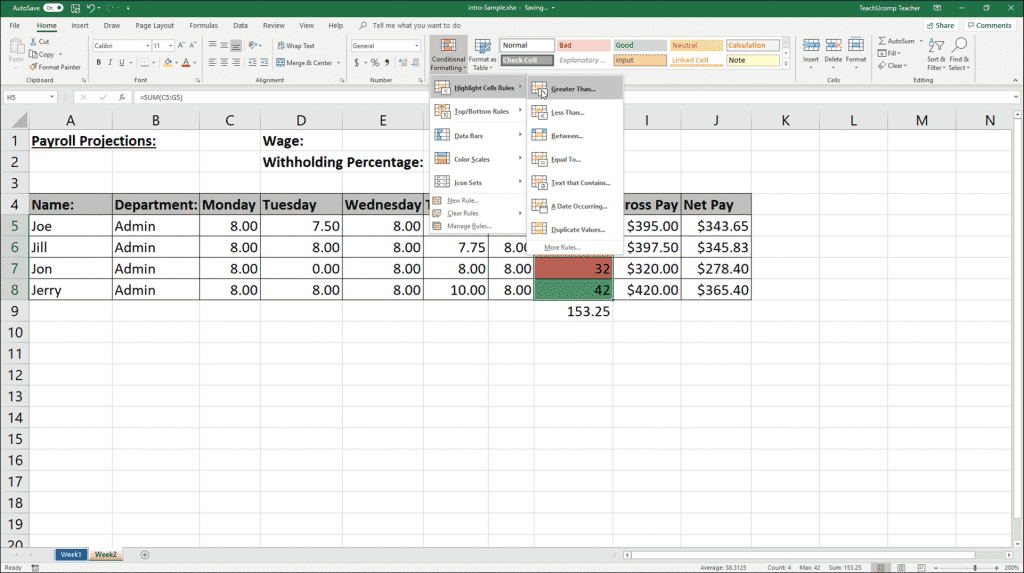
Conditional Formatting in Excel – Instructions: A picture of a user selecting a custom conditional formatting choice from the “Conditional Formatting” button’s drop-down menu.

You can also create multiple rules for selected cells. However, to do this, it’s best to begin by selecting the cells to which to apply multiple conditional formatting rules. Then click the “Conditional Formatting” button in the “Styles” button group on the “Home” tab of the Ribbon. Then choose the “Manage Rules…” command from the drop-down menu that appears to open the “Conditional Formatting Rules Manager” dialog box.

To only view the conditional formatting rules for the selected cells, choose the “Current Selection” choice from the “Show formatting rules for:” drop-down at the top of this dialog box. Otherwise, you can choose to view the conditional formatting rules for the whole worksheet or the entire workbook from this drop-down. Any conditional formatting rules for the selected area then appear in the rules list below that. If you haven’t created any rules for the selected area yet, then this list is blank.

To create a new rule for the selected area, click the “New Rule…” button at the top of the “Conditional Formatting Rules Manager” dialog box. In the “New Formatting Rule” dialog box, select the rule type to create from the “Select a Rule Type:” list. Then enter its evaluation criterion into the area at the bottom of this window. Then choose the formatting to apply when this criterion is met and click the “OK” button to return to the “Conditional Formatting Rules Manager” dialog box.

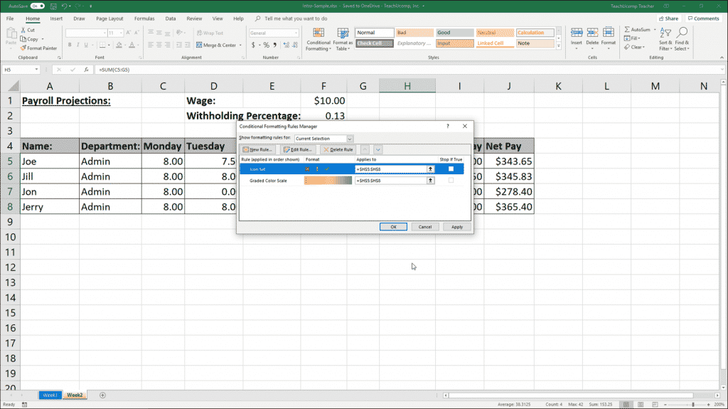
Conditional Formatting in Excel – Instructions: A picture of multiple conditional formatting rules shown within the “Conditional Formatting Rules Manager” dialog box.

To add other rules to the selection, just repeat the process. New rules are added to the list in the “Conditional Formatting Manager” dialog box. If applying multiple rules, they are enforced in the order they appear, from top to bottom, within this dialog box. To change a rule’s order in this list, click to select a rule in this dialog box. Then click the “Move Up” and “Move Down” arrow buttons. For any listed rule, you can check the “Stop If True” checkbox at its right end to end the sequence of rule processing if the cell value meets the criteria specified by the selected rule.

To edit a rule you applied, select it from the list in the “Conditional Formatting Rules Manager” dialog box. Then click the “Edit Rule…” button at the top of the “Conditional Formatting Rules Manager” dialog box to reopen the rule in the “Edit Formatting Rule” window. Change its criterion or formatting and then click the “OK” button. To delete a rule in the “Conditional Formatting Rules Manager” dialog box, select it. Then click the “Delete Rule” button at the top of the “Conditional Formatting Rules Manager” dialog box.

After you finish creating, editing, reordering, or deleting your rules, click the “OK” button in the “Conditional Formatting Rules Manager” dialog box to apply your changes.